Sensitivity and Risk: Stress-Testing the Business Case

Part 9 of 10 in Cobler's Energy Management: The Economics of Saving Energy course. New here? See the course page.

Part 8 built a cash-flow model for the office tower measure set and got one answer: an NPV of about RM956,500. When you plan a drive to a meeting, you rarely ask only "how long does it take?" You also ask "and if the traffic is bad?", because the answer decides when you leave. A business case needs the same second question, because that RM956,500 rests on assumptions: how much demand the BMS really holds off, what the AFA does, how fast tariffs rise, what discount rate the finance team uses, and what the work really costs.

This part tests those assumptions, using the same Part 8 model. We change them one at a time, then in realistic bundles, then pair each real risk with an action. At the end we look at how to choose between several good projects when the budget covers only one. If NPV, IRR and payback still feel unsteady, revisit Part 5 and Part 6 of this course first, because this part changes the inputs and watches those numbers move.

Why one number is not enough

Imagine presenting "NPV = RM956,500" to the board and nothing else. The first sharp question, "and what if the demand limiting only holds off 60 kW, not 100?", leaves you guessing. Sensitivity analysis is asking those questions yourself, in advance, and answering them with the model.

It has three layers, and each answers a different question:

• One-at-a-time (OAT) sensitivity: which single input matters most?
• Scenario analysis: what does a realistic bad case, or good case, look like when several inputs move together?
• Risk and mitigation: what could go wrong, and what will we do about it?

As a reminder, the Part 8 base case is: capex RM130,000 in Year 0; Year 1 savings of RM50,941 (energy, M1 and M2) and RM107,124 (demand, M3); M&V and upkeep RM8,000 a year; electricity savings escalating 2% a year from Year 2 and upkeep 3%; 10 years; 8% nominal discount rate. Base NPV: about RM956,500. Our example office tower is fictional and on the MV non-domestic General tariff.

Change one input at a time

OAT sensitivity holds everything fixed except one input, moves that input to the low or high end of a range you can defend, and records how far NPV moves. We express the move as a percentage of the base NPV:

$$\text{Sensitivity} = \frac{\Delta \text{NPV}}{\text{NPV}_{\text{base}}} \times 100\%$$

Here \(\Delta \text{NPV}\) ("delta NPV") is the change in NPV, and \(\text{NPV}_{\text{base}}\) is the base-case NPV.

Worked example 1: the demand saving. Part 3 gave M3 a range of 60 to 120 kW, with 100 kW as the central estimate. At 60 kW, the demand saving falls by 40 kW × RM89.27 × 12 = RM42,850 in Year 1. In the model that loss also grows 2% a year, like the saving it replaces. Rerunning the Part 8 table with the lower figure lowers the NPV by about RM310,900. (A shortcut gives the same answer: at 8% with 2% growth over 10 years, each ringgit of Year 1 saving is worth about 7.256 ringgit today.)

$$42{,}850 \times 7.256 \approx \text{RM}310{,}900$$

$$\frac{-310{,}900}{956{,}500} \times 100\% \approx -32.5\%$$

Worked example 2: the capex. A 30% cost overrun adds RM39,000. It happens once, in Year 0, so it is not discounted:

$$\frac{-39{,}000}{956{,}500} \times 100\% \approx -4.1\%$$

For this measure set, a shortfall in the demand saving moves the NPV about eight times as much as a large cost overrun. The build cost is small next to the savings, and the demand saving is the largest savings line.

Rank the inputs in a tornado diagram

Do the same for every important input, each across its own range, and list the results from the widest swing to the narrowest. Drawn as horizontal bars, the widest at the top, this is called a tornado diagram, because of its shape.

Choose ranges you can defend, not a flat ±10% for everything. Here the savings ranges come from the low and high estimates in Part 3, the capex range is a ±30% overrun or saving, and the discount rate range is 5% to 12%.

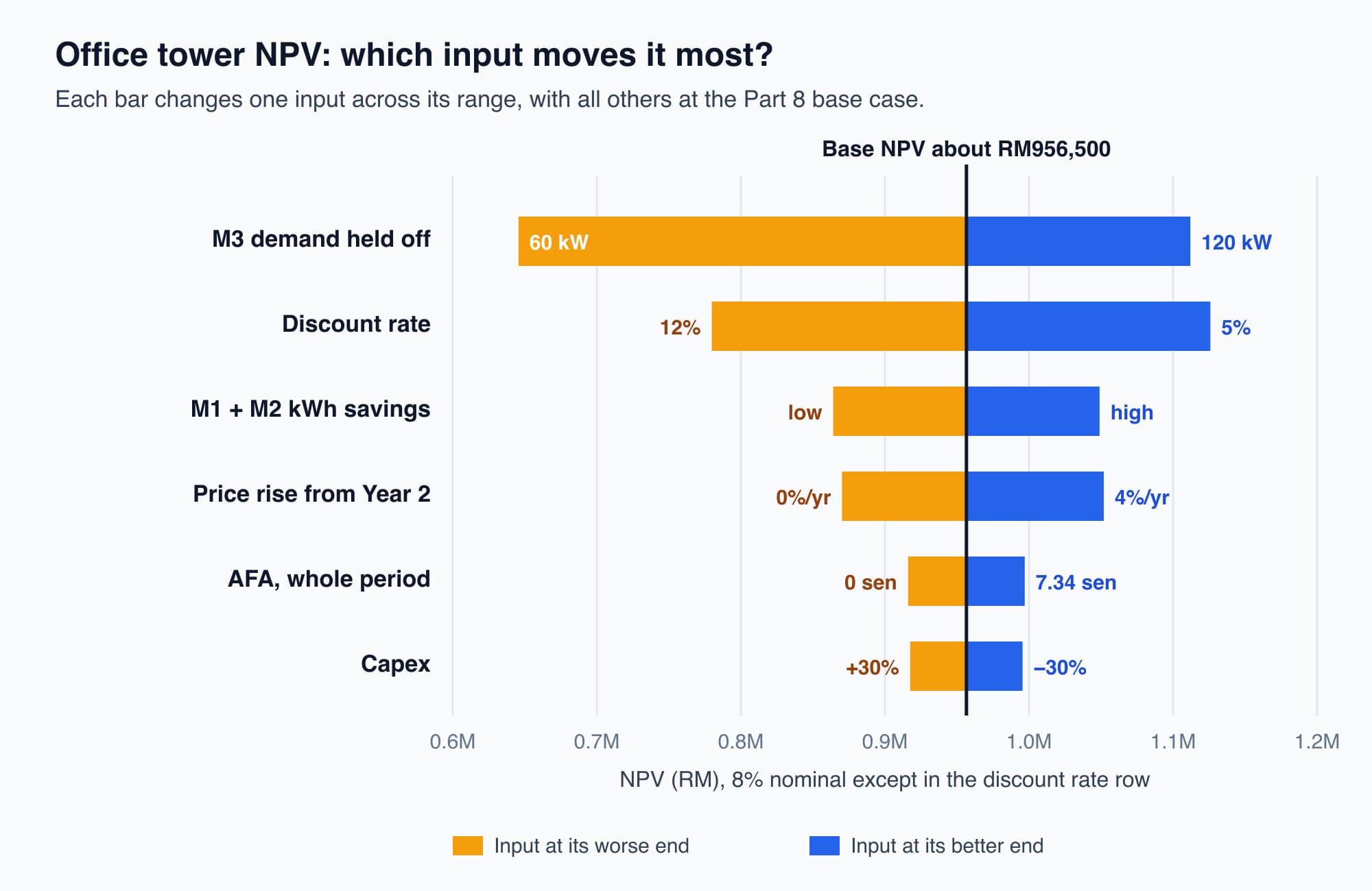
The tornado for the office tower measure set: the demand saving and the discount rate move the NPV most; capex moves it least.

Three points about the ranges:

• The AFA row. Part 2 used the September 2026 AFA (+3.67 sen/kWh) for every month, which is an assumption, because the AFA changes monthly. The row tests an average AFA anywhere from zero to twice September's figure. It changes only the energy saving, because the AFA is charged per kWh.
• The electricity price row. Year 1 (2027) is inside the RP4 tariff period, so only Years 2 to 10 change.
• No row for carbon. A shadow carbon price is not cash, so it is not in the NPV and has no bar. Report the carbon value separately.

The tornado tells you where to spend your effort. For this measure set, the most useful work is proving that the demand limiting really lowers the monthly peak, and agreeing the discount rate with finance early. Tightening the capex quote by a few thousand ringgit barely changes the answer. (A project that saves only kWh, such as lighting, would have a different tornado, with the tariff and hours near the top. Draw it fresh for each project.) If you want to test the demand side yourself, our maximum-demand calculator shows how a lower peak changes the monthly charge.

What if the biggest input fails completely?

The tornado raises a sharper question: what if M3 delivers nothing at all, for example because tenants override the sequence on hot afternoons? Set the demand saving to zero, keep the RM35,000 spent on M3 in the capex, and rerun the model:

• NPV falls from about RM956,500 to about RM179,200.
• Simple payback stretches from about 10 months to about 3.0 years (RM130,000 ÷ (RM50,941 − RM8,000)).

The project still makes money, but most of its value has gone. That is useful to know before you sign. It tells you the demand saving deserves the closest M&V attention, which is why the Part 4 plan checks each month's MD against the BMS log of the kW held off.

Scenarios: move several inputs together

OAT moves one input at a time, but a real bad year often brings several problems at once. Scenario analysis groups a consistent set of assumptions into named cases, usually three:

• Low case: NPV about RM458,300. All three measures at their Part 3 low estimates (RM102,480 a year of savings), capex 30% over budget (RM169,000), and no electricity price rise after Year 1. Simple payback about 1.8 years.
• Medium case: NPV about RM956,500. The Part 8 base case, the one you plan around.
• High case: NPV about RM1,204,400. All three measures at their high estimates (RM192,226 a year), capex on budget, and the 2% price rise.

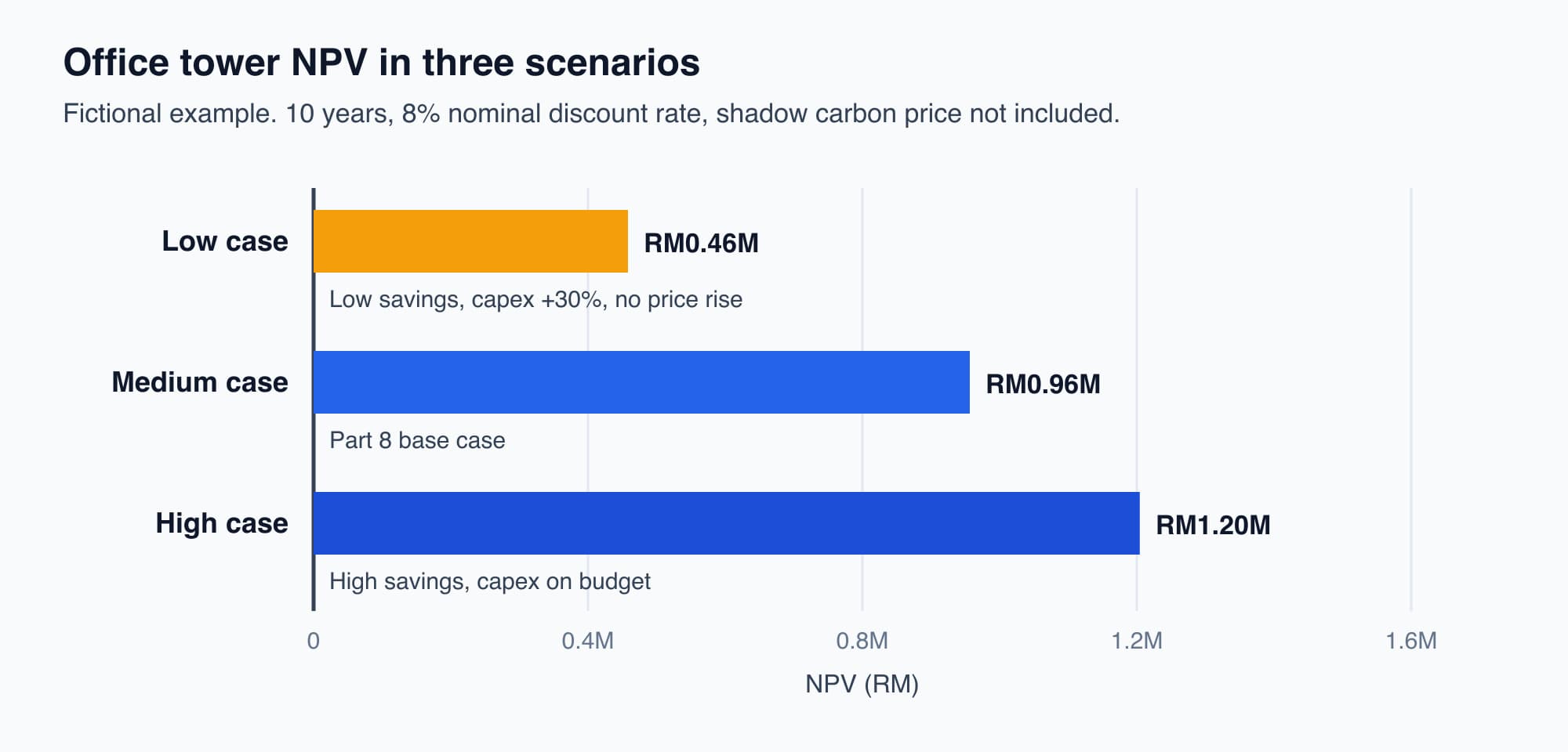
Even the low case stays well above zero, so the measure set makes money across the whole plausible range.

This gives the board a stronger message than one figure: "Across a plausible range from about RM0.46 million to RM1.20 million, this measure set does not lose money." If the low case had gone negative, that would also be useful. It would tell you the project works only if things go well, and you would tighten the weakest assumption before committing.

Pair each risk with a mitigation

Sensitivity tells you how much an input matters. Risk management decides what you will do about it. Pair every material risk with a concrete action:

• The demand limiting does not hold the peak (M3). Test the sequence through a hot month before handover (this is already in the M3 capex), and check each month's MD against the BMS log, as the Part 4 plan requires.
• Tariff and AFA changes. Show the AFA and price-rise rows from the tornado in the business case, so nobody is surprised when the monthly AFA moves.
• Capex overrun. Build a 10 to 15% contingency into the budget from the start, rather than finding the overrun later as a variance.
• Savings fade over time. Apply a degradation factor: assume savings fall 1 to 2% a year as schedules drift and equipment ages. At 2% a year, the office tower NPV falls from about RM956,500 to about RM868,600.

Each mitigation changes the model a little: the contingency raises capex, and the degradation factor trims savings. Applied honestly, they move the medium case slightly towards the low case. A business case that still works after its own mitigations is one you can defend.

Choosing one project from several

Sensitivity tests one project. A different problem arises when you have three good projects, all with positive NPV, and budget for only one. NPV alone may not decide it, because the projects are strong in different ways. You need to weigh several criteria at once, with a multi-criteria decision matrix.

The method has three steps:

1. Normalise each measure onto a common 1 to 10 scale (10 = best), so that a payback in years and an NPV in ringgit can be compared.
2. Weight each criterion by how much it matters to your organisation. One reasonable default is NPV 30%, IRR 20%, Payback 20%, Carbon 20%, Risk 10%.
3. Score each project as the weighted sum, then rank them.

The weighted score is:

$$S = \sum_{i} w_i \times s_i$$

where \(w_i\) is a criterion's weight and \(s_i\) is the project's normalised 1 to 10 score on it. Here is a separate example, three candidates on a Malaysian factory site:

• Project A: LED lighting retrofit (balanced all-rounder)
• Project B: high-efficiency chiller replacement (large, big carbon saving, slow payback, higher risk)
• Project C: compressed-air and steam leak-repair programme (cheap, fast payback)

Working out Project C's total shows the arithmetic:

$$S_C = (0.30 \times 7.2) + (0.20 \times 9.5) + (0.20 \times 9.5) + (0.20 \times 5.0) + (0.10 \times 7.0) = 7.66$$

Project C wins at 7.66, ahead of A (6.78) and B (5.93). The leak repair is not the largest project. The chiller has a larger NPV and a much larger carbon saving. But C's high IRR, very short payback and low risk give it the highest weighted score.

It also helps to score ease of implementation from 1 to 10 alongside risk, because a project you can deliver beats one that stalls. For example: leak repair 9 (a few valves and a weekend), LED retrofit 8 (swap fittings, little disruption), chiller replacement 2 (major plant, downtime, long procurement). The easy, cheap measures are usually the ones to do first, which is also what the optional side reading on the abatement cost curve shows from the carbon side.

The winner changes with the weights

The ranking reflects your priorities; it is not a fixed fact about the projects. Rerun the same table for a firm with a hard carbon target, weighted NPV 20%, IRR 10%, Payback 10%, Carbon 50%, Risk 10%:

• Project B: 7.28
• Project C: 6.54
• Project A: 6.48

Now Project B, the chiller, wins. Nothing about the projects changed, only what the firm decided to value. A business short of cash would reasonably pick C; a business focused on cutting carbon would reasonably pick B. The method makes you state your priorities as numbers before the answer appears. Run the matrix at two or three sets of weights and show the board how the winner moves. If your preferred project wins under only one convenient set of weights, that is worth knowing.

What comes next

You now have the office tower's cash-flow model and a clear view of how far its answer can move. Part 10, Making the Case: A Full Energy Project Appraisal, Start to Finish, puts everything together into a one-page recommendation for management, including the M&V plan that will prove the savings.

The stress tests are also easier when the savings assumptions come from measured data rather than a one-off spreadsheet. Interval readings from the building's meters, the kind we cover in how electricity meters work, let you replace a guessed degradation factor with a measured one and check each month whether the top bar of the tornado is holding up.

Check your understanding

1. In the office tower case, why does a 30% capex overrun change the NPV by only about 4%, while M3 at 60 kW instead of 100 kW changes it by about a third? The overrun is RM39,000, paid once in Year 0. The demand shortfall is RM42,850 in Year 1 and grows every year for ten years, so its present value is about RM310,900. A loss that repeats every year outweighs a one-off cost of a similar size.
2. Why is there no bar for the shadow carbon price in the tornado? Because the shadow carbon price is not cash, so it is not part of the NPV. Changing it would not move the NPV at all. The carbon value is reported on a separate line.

Recap: One NPV hides how fragile it is; a range shows it. One-at-a-time sensitivity finds the inputs that move the NPV most, and a tornado diagram ranks them. For the office tower measure set, the M3 demand saving and the discount rate matter most and capex least. Even if M3 delivers nothing, the NPV stays positive at about RM179,200. Scenarios show a plausible range of about RM0.46 million to RM1.20 million. Each risk gets a mitigation, and a weighted decision matrix helps you choose between projects while showing how the winner depends on your priorities.

This is Part 9 of 10 in Cobler's Energy Management: The Economics of Saving Energy course. Previous: Building an Energy Project Cash-Flow Model. Next: Making the Case: A Full Energy Project Appraisal, Start to Finish.

Cobler builds CobiNeural, a platform that shows a facility team its building's energy, water and indoor air data as live numbers across the whole site. To see how your building performs, talk to us.