From Kilowatt-Hours to Ringgit and Tonnes of CO₂

Part 2 of 10 in Cobler's Energy Management: The Economics of Saving Energy course. New here? See the course page.

Part 1 turned one saving in our example shoplot into ringgit and carbon, and noted that a saved kWh in a large medium-voltage building is worth less than the average price on its bill. Every energy efficiency idea eventually has to answer two questions from the person holding the budget: how much money does it save each year, and how much carbon does it avoid? The money is the kilowatt-hours saved multiplied by the price of only those bill lines that actually fall, which on a medium-voltage bill is often about half the average price per kWh. The carbon is the kilowatt-hours saved multiplied by the grid emission factor.

Payback, net present value and every later figure in this course are built on these two numbers, so an error here carries through to all of them. This part sets out a six-stage method and then applies it to three measures that the facility team has proposed for our example office tower, a fictional 20-storey building on the MV (medium voltage) non-domestic General tariff. The results become the running case for the rest of the course.

Start from real load and real hours

The saving always starts as energy: kilowatt-hours (kWh) that no longer flow through the meter. To estimate it, you need the power the equipment really draws, in kilowatts (kW), and the hours it really runs. Energy is power multiplied by time. If that feels shaky, Power vs Energy: kW and kWh explained in the Electricity Fundamentals course covers it.

The most common mistake is to use the nameplate instead of the real load. Each condenser water pump in our tower has a nameplate that says 30 kW. That is the motor's rated output at full load. A meter on the pump's cable shows it drawing 27.0 kW of electrical input while it runs, and that measured input is what adds up to kWh on the bill. Hours need the same care: a pump that runs 11 hours a day on working days does not run all 8,760 hours of the year.

Real load and real hours come from metered data: half-hourly readings from the main meter or from sub-meters on the equipment. Part 3 shows how to check that data against the bills before using it.

Follow the same six stages for every measure

Here is the method. Every worked example below follows these six stages in order.

1. Baseline power and energy: the "before" case, at real load over real hours.
2. Post-measure power and energy: the "after" case over the same hours.
3. ΔE (delta E): the annual energy saved, the difference between the two.
4. Ringgit: ΔE multiplied by the value of a saved kWh for your tariff, plus any demand saving. The next sections explain both.
5. CO₂: ΔE converted to megawatt-hours (MWh) and multiplied by the grid emission factor, explained in the section on carbon below.
6. Payback: the capital cost divided by the annual ringgit saving. Part 5 covers this properly.

The energy saving is:

$$\Delta E = \left( P_\text{baseline} - P_\text{post} \right) \times \text{annual operating hours}$$

where $P$ is real operating power in kW, not the nameplate. Money and carbon follow from ΔE:

$$\text{Annual saving (RM)} = \Delta E \times \text{tariff (RM/kWh)}$$

$$\text{CO}_2 \text{ avoided (tonnes)} = \frac{\Delta E}{1{,}000} \times \text{EF}_\text{grid}$$

Here "tariff" means the value of a saved kWh, which the next section explains, and EF is the grid emission factor in tonnes of CO₂ per MWh. Dividing kWh by 1,000 gives MWh. Part 5 then uses:

$$\text{Payback (years)} = \frac{\text{Capex (RM)}}{\text{Annual saving (RM/yr)}}$$

A saved kWh is worth only the bill lines that fall

The easy way to value a saved kWh is to divide the whole bill by the whole kWh. For the tower's September 2026 bill on the MV non-domestic General tariff, that is RM310,532 ÷ 500,000 kWh = 62.1 sen/kWh. This is the average, or blended, rate. It is the wrong number for valuing a kWh saving, because not every line of the bill falls when you use fewer kWh.

Go through the tower's bill line by line (Your TNB Bill, Line by Line, in the bill course, explains each one):

• Energy, 29.83 sen/kWh: falls with every kWh saved.
• AFA (Automatic Fuel Adjustment), +3.67 sen/kWh in September 2026: also charged per kWh, so it falls too.
• Capacity and network, RM89.27 per kW of maximum demand (MD): these depend on the highest half hour of the month. They fall only if that half hour falls.
• Retail, RM200 a month: fixed. It never falls.

So each kWh the tower saves is worth 29.83 + 3.67 = 33.50 sen, unless the saving also lowers the monthly peak. This is called the marginal value: what the bill loses when one more kWh is saved. It is little more than half of the 62.1 sen blended rate.

A low-voltage (LV) building is different. Our example shoplot is on LV non-domestic General, where capacity (8.83 sen) and network (14.82 sen) are charged per kWh, not per kW. So a saved kWh removes 27.03 + 8.83 + 14.82 + 3.67 = 54.35 sen. Its blended rate, RM4,368 ÷ 8,000 kWh = 54.6 sen, is almost the same, because only the RM20 retail charge is fixed.

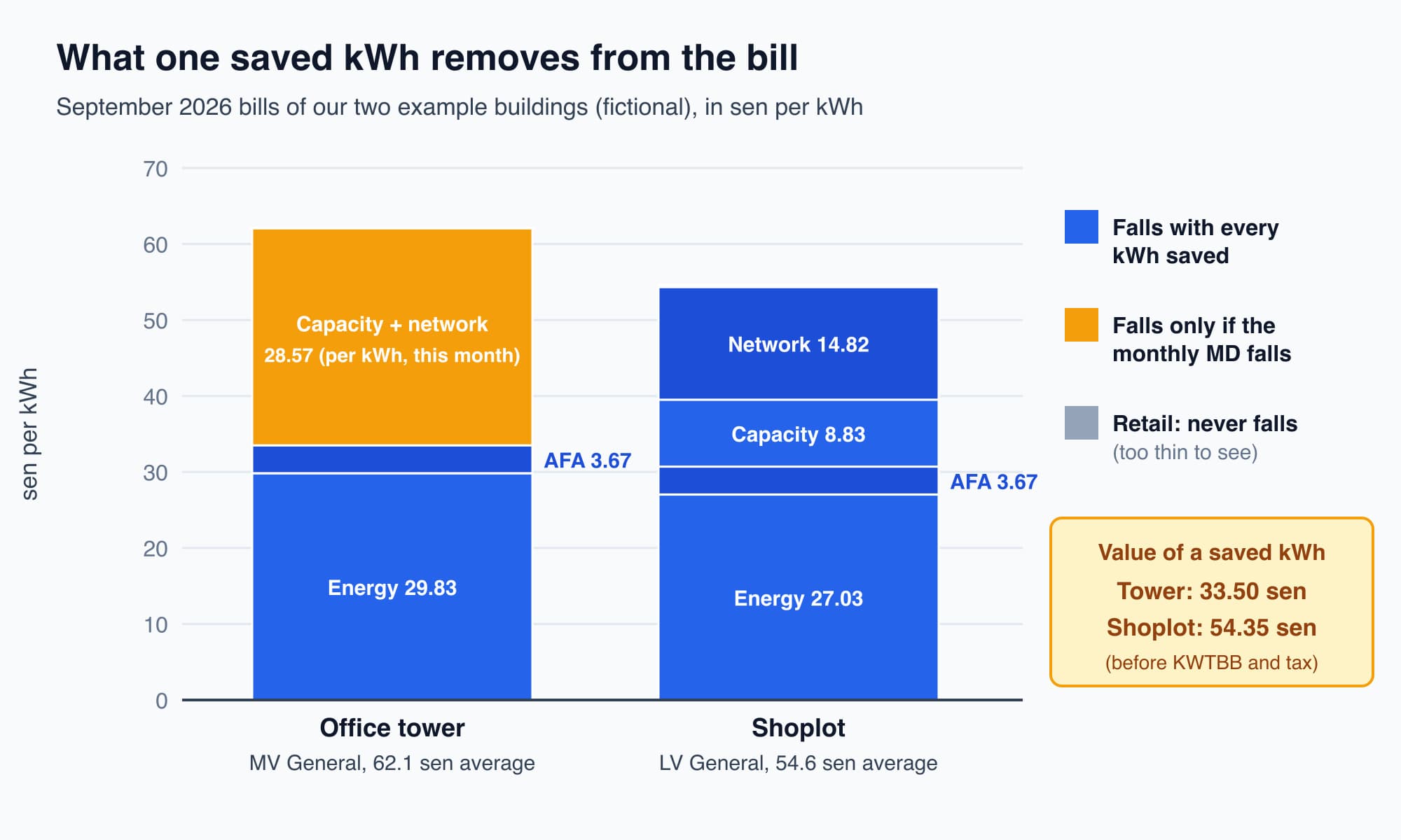
On the tower's MV bill, capacity and network (orange) fall only if the peak falls; on the shoplot's LV bill, almost every line falls with each saved kWh.

Three notes on these rates:

• AFA changes monthly. We use September 2026's +3.67 sen for a whole year of savings. That is an assumption, and a different AFA would change the result.
• KWTBB and tax are left out. The KWTBB levy is 1.6% of the energy and demand charges (Your TNB Bill, Line by Line), so it would add a little to each saving. We leave it out to keep the numbers simple and slightly conservative.
• On a Time-of-Use (ToU) tariff, timing matters. On MV ToU, a kWh saved in the weekday peak window is worth 31.32 + 3.67 = 34.99 sen, and one saved off-peak is worth 27.23 + 3.67 = 30.90 sen (Time-of-Use, Green Tariffs and Avoidable Penalties explains the windows).

Count a demand saving only if the monthly peak falls

On an MV bill, a measure can save money in a second way: by lowering the maximum demand. On MV General, each kW off the month's highest half hour saves RM89.27 that month (Maximum Demand: Why One Bad Half-Hour Costs So Much explains how the charge is set). Trimming demand can be worth more than the energy it saves. Our maximum demand calculator puts a ringgit figure on a kW reduction.

The condition is strict. A demand saving counts only if the highest half hour of the month really falls. Using less power at some other time of day does nothing to the demand charge. For the tower, whose MD is usually set on a hot weekday afternoon around 2:30pm:

• A measure that saves power at 7pm does not lower the MD, because the tower's MD is not set at 7pm.
• A measure that saves power on mild mornings but not in the hottest half hour does not lower the MD either.
• A measure aimed at the top half hours can lower it, and the saving is the kW removed from each month's peak × RM89.27 × 12 months, if it works every month.

Two other items are worth checking but are not part of the kWh value. A measure that improves power factor can remove a surcharge (see Power Factor Correction: What Capacitor Banks Do); that saving is valued separately. On MV ToU, only the peak-window MD is charged, at RM97.06 per kW.

Convert the kWh saved into carbon

The carbon calculation uses the grid emission factor: the average CO₂ released for each kWh generated on the grid. For Peninsular Malaysia it is 0.740 kg CO₂e per kWh, the same as 0.740 tonnes per MWh (Suruhanjaya Tenaga, 2024 figure, provisional, published 23 February 2026). Sabah (0.539) and Sarawak (0.199) have their own factors. How to calculate Scope 2 emissions in Malaysia explains where these come from.

Two cautions apply:

• 0.740 is an average for the whole grid. The power stations that actually cut back when you save a kWh may emit more or less than the average. The average is the standard figure for reporting, but it is an approximation of the carbon a saving avoids.
• Carbon follows kWh, not kW. A measure that only moves load to another half hour saves no kWh, so it avoids no carbon, even if it saves money on the demand charge.

Value the tower's three measures

The tower's facility team has proposed three measures, based on sub-meter readings and the building's schedules. Here we value the team's central estimates; Part 3 checks them against a full baseline and puts a low and high value on each. The tower is on MV non-domestic General, so each saved kWh is worth 33.50 sen, and the working year has 22 working days a month, 264 in all.

M1: stop the chiller plant at 6pm instead of 8pm. The plant draws about 220 kW in those two hours, less about 20 kW for tenants who request cooling after 6pm. So the power falls by 200 kW for 2 hours on each working day, which is 2 × 264 = 528 hours a year.

• ΔE = 200 kW × 528 h = 105,600 kWh a year.
• Ringgit: 105,600 × RM0.3350 = RM35,376 a year.
• CO₂: 105,600 ÷ 1,000 × 0.740 = 78.1 tonnes a year.
• Demand: none. The plant is already running at 2:30pm, and nothing changes then.

M2: variable speed drives (VSDs) on the two condenser water pumps. Before, the two pumps draw 2 × 27.0 = 54.0 kW. After, they are expected to average 2 × 19.0 = 38.0 kW. They run together from 7am to 6pm, 11 hours on each working day, so 11 × 264 = 2,904 hours a year.

• ΔE = (54.0 − 38.0) × 2,904 = 16 × 2,904 = 46,464 kWh a year.
• Ringgit: 46,464 × RM0.3350 = RM15,565 a year.
• CO₂: 46,464 ÷ 1,000 × 0.740 = 34.4 tonnes a year.
• Demand: none counted. In the hottest half hour the pumps run close to full speed, so the peak barely changes.

Notice the hours for M2. Before M1, one condenser pump also ran with the plant from 6pm to 8pm. M1 removes those hours, so M2 must not count them again. Valuing M2 on the old running hours would have claimed an extra 8 kW × 2 h × 264 = 4,224 kWh a year that M1 already saves. When two measures touch the same equipment, value the second on what is left after the first.

M3: BMS demand limiting in the top half hours. The building management system (BMS) holds off the car park ventilation fans, the water transfer pumps and a small chilled water temperature reset for the few half hours near the peak. The loads run a little later, so the energy is moved, not removed.

• ΔE: 0 kWh counted.
• Demand: 100 kW off each month's MD × RM89.27 × 12 = RM107,124 a year.
• CO₂: 0 tonnes, because no kWh are saved.

The measure set is worth about RM158,065 a year and 112.5 tonnes of CO₂e a year at September 2026 prices, before KWTBB and tax. Using the low and high estimates that Part 3 sets out gives about RM102,480 to RM192,226 a year.

Now compare the blended-rate shortcut. At 62.1 sen, M1 would appear to save 105,600 × 62.1 sen, or about RM65,600 a year. That is about 85% more than it really saves. The same shortcut would give M3 nothing at all, because M3 saves no kWh. The blended rate overstates the kWh measures and misses the demand measure.

The table also shows where the risk sits. About two-thirds of the value (RM107,124 of RM158,065) comes from M3, and M3 pays only in months when the peak really falls. Part 4 sets out how each measure will be checked, and Part 9 tests what happens if M3 delivers less.

The same method for a low-voltage building

The method works the same way on an LV bill, but the value per kWh is higher. Suppose a warehouse on LV non-domestic General has 300 light fittings at 72 W each, lit for 3,000 hours a year. Replacing each with a 30 W LED fitting giving the same light costs RM55,000 installed.

Baseline power, 72 W across 300 fittings:

$$P_\text{baseline} = 300 \times 0.072 = 21.6 \text{ kW}$$

Power after the retrofit, at 30 W each:

$$P_\text{post} = 300 \times 0.030 = 9.0 \text{ kW}$$

The saving is 42 W per fitting, or 12.6 kW in total, over 3,000 hours:

$$\Delta E = (21.6 - 9.0) \times 3{,}000 = 12.6 \times 3{,}000 = 37{,}800 \text{ kWh/yr}$$

On LV General each saved kWh is worth 54.35 sen, so the retrofit saves 37,800 × RM0.5435 = RM20,544 a year (RM20,544.30). The carbon is 37.8 MWh × 0.740 = 28.0 tonnes of CO₂e a year. Because an LV bill has no per-kW charge, there is no separate demand saving to check.

When the saving is fuel, not electricity

Not every measure saves electricity. Recovering waste heat, tuning a boiler or insulating steam pipes saves fuel. The six stages still apply, but the money comes from the fuel price and the carbon from the fuel's own emission factor:

$$\text{CO}_2 = \text{fuel saved} \times \text{EF}_\text{fuel}$$

This course does not give a gas price or gas emission factor, because we have not yet verified current Malaysian figures. Take the price, period and energy content from your supplier's contract, use an authoritative emission factor on the same basis (per cubic metre or per gigajoule), and never apply the grid factor to fuel. Industrial readers can see the optional side reading, Fuel, Heat and Why Thermal Savings Are the Big Money.

What comes next: checking the estimates against a baseline

We now have a value for each measure: RM158,065 and 112.5 tonnes a year for the tower. These values rest on a few readings: the plant's draw after 6pm, the pumps' steady 27.0 kW and the half hours near the peak. Before anyone relies on them, they need checking against a full record of how the building uses energy through the year. The next part, Before You Claim Savings: Baseline and Load Profile, builds that baseline from twelve bills and half-hourly data, shows where the three measures come from and puts a range on each.

Check your understanding

1. A measure in our example office tower saves 10,000 kWh a year, all at night, and does not change the MD. What is it worth in ringgit and carbon at September 2026 rates? On MV General only energy and AFA fall, so the value is 10,000 × RM0.3350 = RM3,350 a year. The carbon is 10,000 ÷ 1,000 × 0.740 = 7.4 tonnes of CO₂e a year. Using the 62.1 sen blended rate would have overstated the money at about RM6,210.
2. The same 10,000 kWh saving in our example shoplot on LV General is worth more. Why, and how much? On LV General, capacity and network are charged per kWh, so they fall with every kWh saved, along with energy and AFA. The value is 10,000 × RM0.5435 = RM5,435 a year. Only the RM20 retail charge stays fixed.

Recap: Estimate kWh savings from measured power and real running hours, never the nameplate. Value a saved kWh at the rate of the bill lines that actually fall: 33.50 sen on the tower's MV General bill (energy plus September 2026 AFA) and 54.35 sen on the shoplot's LV General bill. Count a demand saving only if each month's peak really falls. Multiply kWh by 0.740 kg CO₂e per kWh for Peninsular Malaysia; moving load saves no carbon. When measures overlap, value each on what the others leave. The tower's three measures are worth about RM158,065 and 112.5 tonnes of CO₂e a year, and about two-thirds of that money depends on the peak falling.

This is Part 2 of 10 in Cobler's Energy Management: The Economics of Saving Energy course. Previous: Why Saving Energy Is Really About Money (and Carbon). Next: Before You Claim Savings: Baseline and Load Profile.

Cobler builds CobiNeural, a platform that shows a facility team its building's energy, water and indoor air data as live numbers across the whole site. To see how your building performs, talk to us.