Building an Energy Project Cash-Flow Model

Part 8 of 10 in Cobler's Energy Management: The Economics of Saving Energy course. New here? See the course page.

Part 7 added up every cost of owning one machine over its life, and a business case needs the same kind of year-by-year list for a whole project. If you have ever planned a big household purchase, you have probably written something like this on paper: what it costs now, what it saves or costs each year after that, and when it will need replacing. A cash-flow model for an energy project is the same list, done carefully, one row for each kind of money and one column for each year.

In the last few parts you met payback, ROI, NPV, IRR and life-cycle cost. Each of them is calculated from this one table. So the natural question is: how do you build the table, and what goes into it? This part answers that step by step, using the office tower measure set you valued in Part 2.

What is a cash-flow model?

A cash-flow model is a year-by-year table of every ringgit a project moves. It starts at Year 0, the day you pay for the work, and runs to the end of the period you are judging, here Year 10. Money coming in (savings) is positive. Money going out (costs) is negative.

Every metric from the earlier parts reads this table in a different way:

• Simple payback asks when the running total of cash turns positive.
• NPV discounts each year's cash to today's value and adds them up.
• IRR finds the discount rate at which that NPV would be zero.

If the table is right, all three are right. If one cell is wrong, for example a forgotten upkeep cost, every metric you show the board is wrong in the same direction.

The five kinds of money in any energy project

Any energy project, large or small, is built from five kinds of money. Each becomes one row of the table.

1. Capital expenditure (capex). The upfront cost: equipment, installation, engineering and commissioning. It almost always lands in Year 0 and is negative (money out).
2. Operating savings. The reason the project exists: lower electricity bills, including avoided maximum demand (MD) charges where the peak really falls. Positive, and they recur every year the measure works.
3. Operating costs. Any running cost the project adds: extra maintenance, service contracts, and the cost of measuring the saving. Usually small, but real, and negative.
4. Replacement costs. Spending in the middle of the period to keep the measure working, such as a variable speed drive (VSD) that wears out before the analysis ends. Negative, and it arrives in one lump in one year.
5. Terminal (salvage) value. What the equipment is worth at the end. Often zero for equipment built into a building. It appears once, in the final year.

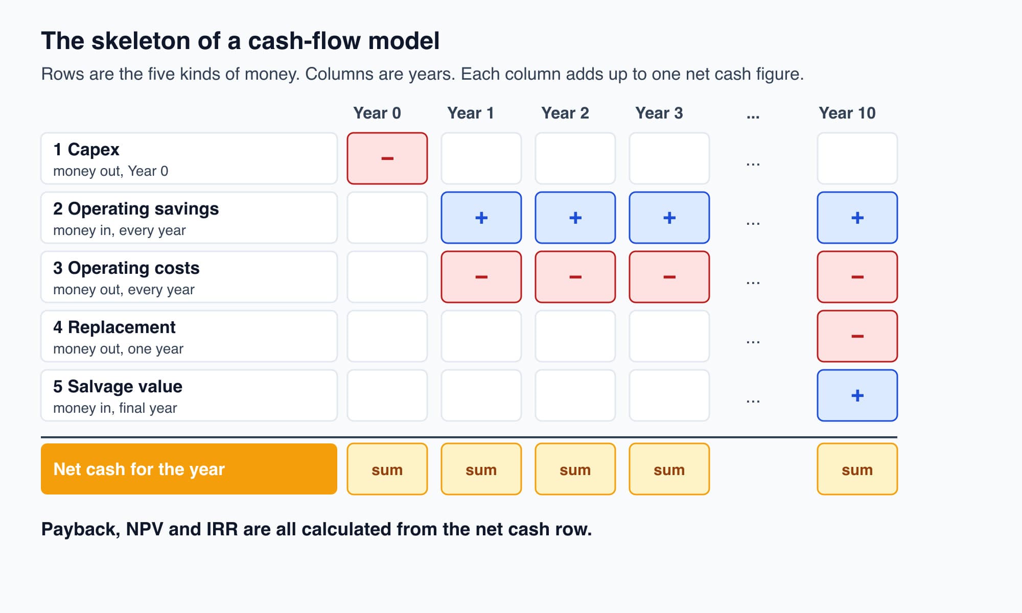
The skeleton of a cash-flow model: five kinds of money as rows, years as columns, and one net cash figure for each year.

Fill in Year 0 and Year 1 for the office tower

Now we fill the skeleton for one real case. In Part 2 we valued three measures on our example office tower (a fictional 20-storey Kuala Lumpur building on the MV non-domestic General tariff):

• M1, chiller plant scheduling: the plant stops at 6pm with the air handling units, instead of running on an old schedule until 8pm. An after-hours request button runs it for late tenants. It saves 105,600 kWh a year.
• M2, VSDs on the two condenser water pumps: 46,464 kWh a year, counted only over the hours left after M1, so the two measures do not claim the same hours twice.
• M3, BMS demand limiting: the building management system (BMS) holds off some load in the highest half-hours. It moves load rather than removing it, so it saves no kWh, but it lowers the monthly MD by 100 kW.

Part 2 valued the kWh at the marginal rate: the energy charge plus the Automatic Fuel Adjustment (AFA), 29.83 + 3.67 = 33.50 sen/kWh, using the September 2026 AFA for every month. The demand saving counts only because the peak really falls: 100 kW × RM89.27 × 12 months. All figures are before the KWTBB (Renewable Energy Fund) levy and tax.

Year 0 (capex). The proposed costs are RM15,000 for M1, RM80,000 for M2 and RM35,000 for M3, a total of −RM130,000. The work is installed from October to December 2026.

Year 1 (2027), savings.

• Energy saving (M1 + M2): 152,064 kWh × 33.50 sen = RM50,941.
• Demand saving (M3): 100 kW × RM89.27 × 12 = RM107,124.

Year 1, operating cost. The M&V plan from Part 4, plus upkeep of the new drives and the demand-limiting sequence, costs about RM8,000 a year.

Replacement. VSDs of this kind are expected to last about 15 years, so no replacement falls inside our 10-year period. The row stays in the model with zeros, so that anyone reading it can see it was considered.

Salvage. The controls changes and drives are built into the plant, so we take the value at Year 10 as RM0.

Netting Year 1:

$$50{,}941 + 107{,}124 - 8{,}000 = \text{RM}150{,}065$$

Notice that the demand saving is the larger of the two savings lines. That is only true because M3 really lowers the peak. If it did not, the RM107,124 would be zero, and Part 9 tests exactly that.

Escalation: why Year 5 is not a copy of Year 1

The most common beginner error is to type the Year 1 saving into one cell and copy it across ten columns. Prices do not stand still. Electricity tariffs change, and labour for maintenance becomes more expensive. Escalation grows each line at its own rate:

$$\text{Value in year } t = \text{Value}_{yr1} \times (1 + g)^{(t-1)}$$

Here \(g\) is the escalation rate for that line, as a decimal (2% is 0.02), and \(t\) is the year number. The \((t-1)\) is there because Year 1 is the starting point, so it has not grown yet. We use \(g\), not \(r\), because \(r\) is kept for the discount rate from Part 6.

For the office tower we assume:

• Electricity savings (energy and demand): 2% a year from Year 2. The RP4 tariff schedule (the TNB tariff structure in force since July 2025) runs to 31 December 2027, so Year 1 (2027) uses today's rates. The 2% after that is an assumption for teaching, not a forecast.
• Operating costs: 3% a year, to follow wages.

A worked example: the demand saving in Year 5 is

$$107{,}124 \times (1.02)^{4} = 107{,}124 \times 1.0824 = \text{RM}115{,}954$$

That is about RM8,800 more than the flat Year 1 figure. Leaving escalation out would understate the later years.

Carbon: count the tonnes, but keep them out of the cash

The measures also cut emissions. To convert kWh to tonnes we use the grid emission factor for Peninsular Malaysia: 0.740 kg CO2e per kWh (2024, provisional, published by Suruhanjaya Tenaga, the Energy Commission). It is an average for the grid, and we hold it constant for all ten years, which is a simplification.

• M1 and M2: 152,064 kWh × 0.740 = 112,527 kg, about 112.5 tonnes CO2e a year.
• M3: no kWh saved, so no carbon claimed.

Some companies put an internal price on each tonne they avoid, called a shadow carbon price. The formula is simple:

$$\text{Carbon value} = \text{tCO}_2 \text{ saved} \times \text{internal carbon price (RM/tCO}_2)$$

At an illustrative internal price of RM50 per tonne, the tower's carbon value is 112.5 × 50 ≈ RM5,630 a year.

That RM5,630 is not cash. Nobody pays the tower RM5,630, and no bill falls by that amount. So it does not go into the net cash row, the payback or the IRR. If your company uses a shadow price, show it on a separate line below the cash-flow table, labelled as a policy value. Malaysia has announced a carbon tax but no rate, as we explain in carbon tax in Malaysia, so a shadow price is a choice your company makes, not a cost it pays today.

The full ten-year table

Now we escalate the recurring lines and lay out the full table. The Year 0 row holds the capex. Replacement and salvage are zero in every year, so we have left those two columns out to keep the table readable. The last column is the present value (PV) of each year's net cash at our discount rate.

About the 8% discount rate. This course uses 8% nominal, an illustrative figure. "Nominal" means it includes expected inflation. It matches our cash flows, which are also nominal: they are the actual ringgit amounts we expect in each year, including the 2% and 3% price rises.

Each PV is the net cash divided by \((1.08)^t\). For Year 1, 150,065 ÷ 1.08 = 138,949.

(Real and nominal, for the curious. Some companies prefer a real model: cash flows in today's prices, with no inflation in them, discounted at a real rate that also has inflation removed. A real rate is roughly the nominal rate minus inflation. Either method is fine if you use it consistently. The mistake is mixing them, for example escalated nominal savings discounted at a real rate, which makes a project look better than it is.)

Read payback, NPV and IRR from the table

Every metric now comes straight from the last two columns.

NPV. Add up the PV column, including the negative Year 0:

$$\text{NPV} = \sum_{t=0}^{10} \frac{\text{Net cash}_t}{(1 + 0.08)^t}$$

The ten years of PVs add to about RM1,086,500, and the capex is −RM130,000, so the NPV at 8% is about RM956,500 (RM0.96 million). In words: after paying for the work and the upkeep, the measure set leaves the owner about RM956,500 better off in today's ringgit than doing nothing.

Payback. The Year 1 net cash (RM150,065) is larger than the capex, so the money comes back inside the first year. If the savings arrive evenly through the year, the simple payback is 130,000 ÷ 150,065 ≈ 0.87 years, about 10 months. Using the PV column instead, the discounted payback is 130,000 ÷ 138,949 ≈ 0.94 years, about 11 months. Always say which one you are quoting.

IRR. The discount rate that would bring the NPV to zero is about 117%. It is this high because the capex is small and the demand saving is large. It is not a typing error, but it also depends heavily on M3 working as planned.

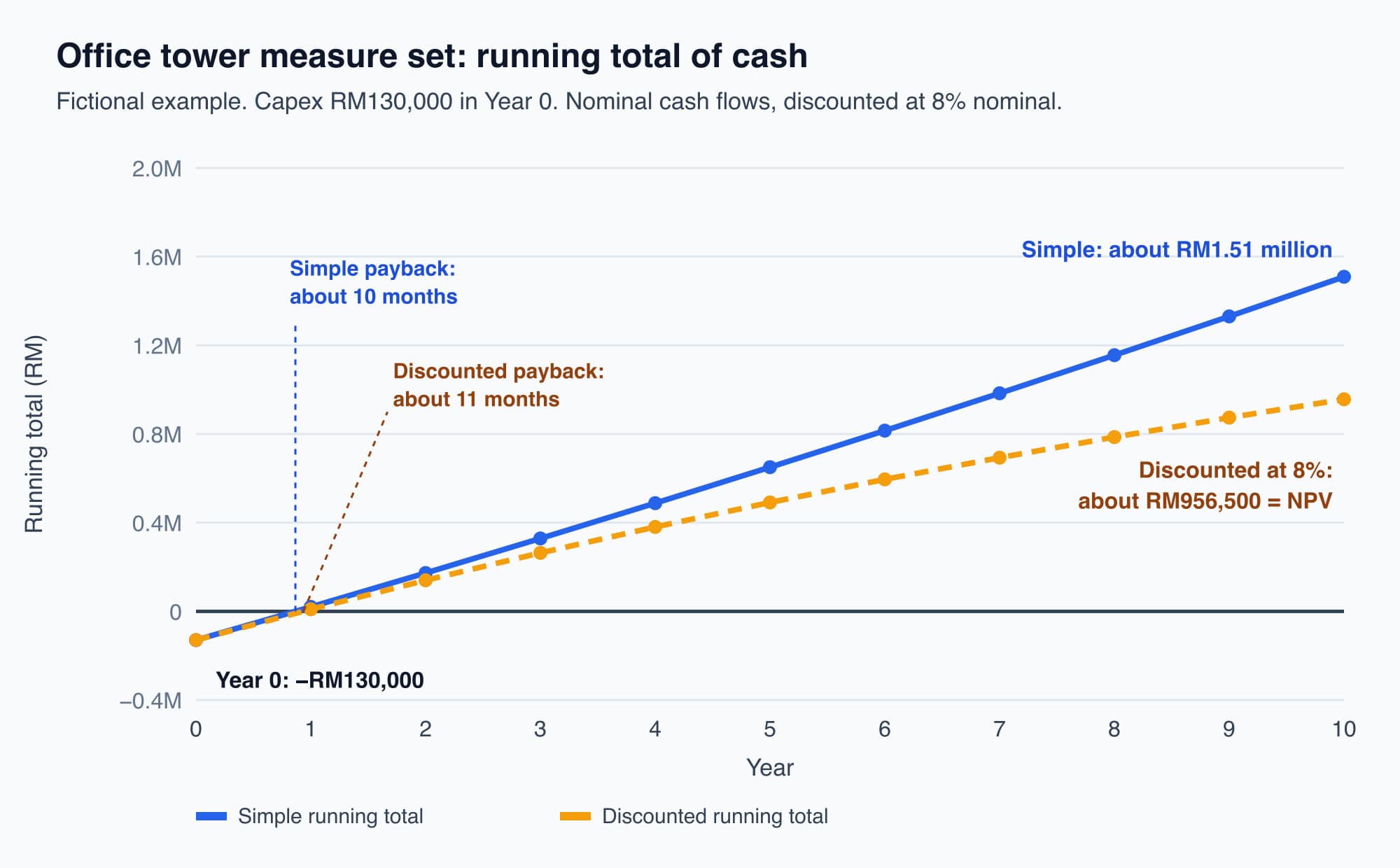
The running total of cash crosses zero within the first year. The discounted line crosses a little later and ends lower, at the NPV of about RM956,500.

Controls measures like these often pay back fast, so a table like this one is common for scheduling and demand-limiting work. A chiller replacement costing millions would cross zero much later, and there the discounting would change the answer far more.

Six mistakes that spoil a model

1. Using the blended (average) tariff instead of the marginal rate. On an MV bill, the average rate includes demand charges that do not fall when only kWh fall. Part 2 showed that valuing M1 at the 62.1 sen blended rate instead of 33.50 sen overstates it by about 85%. If your saving is about when you use power, value the demand part separately, and only if the peak falls. (See how power and energy differ and the maximum-demand calculator.)
2. No escalation, no discounting. Flat lines understate later savings. Leaving out discounting overstates them. You need both.
3. Leaving out upkeep and replacement. A model with only savings is a sales brochure. Include the M&V cost, the maintenance and any mid-life replacement.
4. Counting a shadow carbon price as cash. It makes payback and IRR look better with money that never arrives. Show it separately.
5. Unrealistic operating hours. Savings scale with running hours. Part 2 counted M2 over the 11 hours left after M1. On the old schedule one pump also ran from 6pm to 8pm; counting those hours for M2 as well would have added 4,224 kWh a year that M1 already removes.
6. Typed-in numbers instead of formulas. If a cell says `= 115954`, nobody, including you next year, can check it or rerun it. Each cell should refer to its base and its rate, so one tariff change flows through the whole table.

The last two mistakes are where measurement matters. The model is only as good as the savings and hours going into it, and those are checked against metered data from the meters themselves, which is what the Part 4 M&V plan sets up.

What comes next

The table gives one NPV, about RM956,500, and every number in it rests on an assumption: the demand saving, the AFA, the escalation, the discount rate, the capex. Part 9, Sensitivity and Risk: Stress-Testing the Business Case, changes those assumptions one at a time in this same model and shows which ones could change the decision.

Check your understanding

1. Why does the office tower's shadow carbon value of RM5,630 a year not appear in the net cash row? Because it is not money that arrives. No bill falls by that amount and nobody pays it. Putting it in the cash row would make the payback and IRR look better than the real cash supports. It belongs on a separate line, labelled as a policy value.
2. The Year 1 demand saving is RM107,124. Why is it RM115,954 in Year 5? The model escalates the electricity savings by an assumed 2% a year from Year 2: 107,124 × 1.02⁴ ≈ 115,954. Year 1 uses today's RP4 rates because the tariff schedule runs to the end of 2027.

Recap: A cash-flow model is a year-by-year table of every ringgit a project moves, from Year 0 to the end of the analysis. It has five kinds of money: capex, savings, operating costs, replacement and salvage. Each recurring line is escalated at its own rate, and the cash flows must match the discount rate (nominal with nominal). Carbon tonnes are reported, but a shadow carbon price is kept out of the cash. For the office tower measure set, RM130,000 of capex gives an NPV at 8% of about RM956,500, a simple payback of about 10 months and an IRR of about 117%.

This is Part 8 of 10 in Cobler's Energy Management: The Economics of Saving Energy course. Previous: Life-Cycle Costing: The Cheapest to Buy Is Often the Costliest to Own. Next: Sensitivity and Risk: Stress-Testing the Business Case.

Cobler builds CobiNeural, a platform that shows a facility team its building's energy, water and indoor air data as live numbers across the whole site. To see how your building performs, talk to us.