How a BMS Guards Your Electricity Bill: Load Shedding and Demand Limiting

Part 14 of 16 in Cobler's Building Automation and BMS Fundamentals course. New here? See the course page.

Parts 12 and 13 showed how the building management system (BMS) runs the chiller plant and the air side, which together take the largest share of the office tower's electricity on a hot afternoon. That left a question: how can a BMS trim the building's demand for a few minutes at a time to lower the monthly demand charge? On a hot weekday the chillers, pumps, air handling units, lifts and lights are all busy together, and the busiest half hour is usually 2:30pm to 3:00pm. That one half hour can decide a large part of the month's electricity bill.

A BMS limits demand by watching the building's power during each 30-minute period, and by briefly easing or delaying loads that can wait, so that the half-hour average stays below a limit you choose. This only saves money on a tariff that charges for maximum demand in kW, and when a half hour counts depends on the tariff. This part is the course's one place for how the TNB (Tenaga Nasional Berhad) tariff applies to BMS control.

The bill charges for energy and, on some tariffs, for the busiest half hour

A useful comparison is two cars that each travel 100 kilometres in a day. One drives at a steady pace. The other crawls, then accelerates hard, then crawls again. They cover the same distance, but the second car needs a bigger engine to cope with its bursts. An electricity bill can charge for both things:

• Energy, in kilowatt-hours (kWh), is how much electricity the building used over the month. This is the distance travelled.
• Demand, in kilowatts (kW), is how fast the building was drawing power at its busiest time. This is how hard the driver accelerated.

The Electricity course explains the difference in Power vs Energy: kW and kWh and goes through each line of a bill in Your TNB Bill, Line by Line. Here we only need one idea from those lessons. Two buildings can use the same kWh in a month and pay very different demand charges, because one of them had a much higher peak.

The utility charges for demand because every cable, transformer and power station upstream must be sized for your busiest moment, not your average one. That capacity is reserved for you whether you use it for half an hour or all day.

Which tariffs charge for demand, and which half hours count

Under RP4, the TNB tariff structure in force since 1 July 2025, the demand charge is made of two parts, Capacity and Network, both charged per kW. It applies only to some tariff categories:

LV means low voltage (the 400/230 V supply small buildings take from the street). MV means medium voltage, where a larger building takes an 11 kV supply into its own substation. Time of use (ToU) tariffs charge different energy rates at different times of day. On MV ToU, demand is charged only for the peak window, 2pm to 10pm on weekdays; weekends are off-peak throughout. These totals do not apply to high voltage (HV) or special tariff categories.

The office tower is on MV non-domestic General. Every half hour of the month can set its maximum demand, including early mornings and Saturdays. For contrast, our example shoplot, a fictional three-storey shoplot in Petaling Jaya with a café and a small office, is on LV General, so it has no per-kW charge at all. For the shoplot, the useful saving is total kWh, and demand limiting would not lower its bill.

So before setting up any demand logic, first check which tariff the building is on. You can explore your own numbers with our maximum-demand calculator, and the Economics course covers the demand charge in The Maximum Demand Charge.

Maximum demand is the highest 30-minute average, not a one-second spike

TNB measures maximum demand (MD) as the highest metered 30-minute average kW in the month. The meter works out how much energy the building used in a half hour and turns it into an average power. (Two times the kWh in a half hour gives the average kW, because a half hour is half of an hour.)

Because it is an average, a short burst counts for little. Suppose the building draws an extra 300 kW for 2 minutes. Averaged over 30 minutes, that adds only 300 × 2 ÷ 30 = 20 kW to the half-hour average. A burst that lasts most of the half hour, on the other hand, counts almost in full.

This tells the BMS what to aim for. It does not need to stop every brief surge. It needs to keep each half-hour average below the limit.

Here is Thursday 17 September 2026 in the office tower. The highest half hour, 2:30pm to 3:00pm, reached 1,600 kW, which set the month's maximum demand.

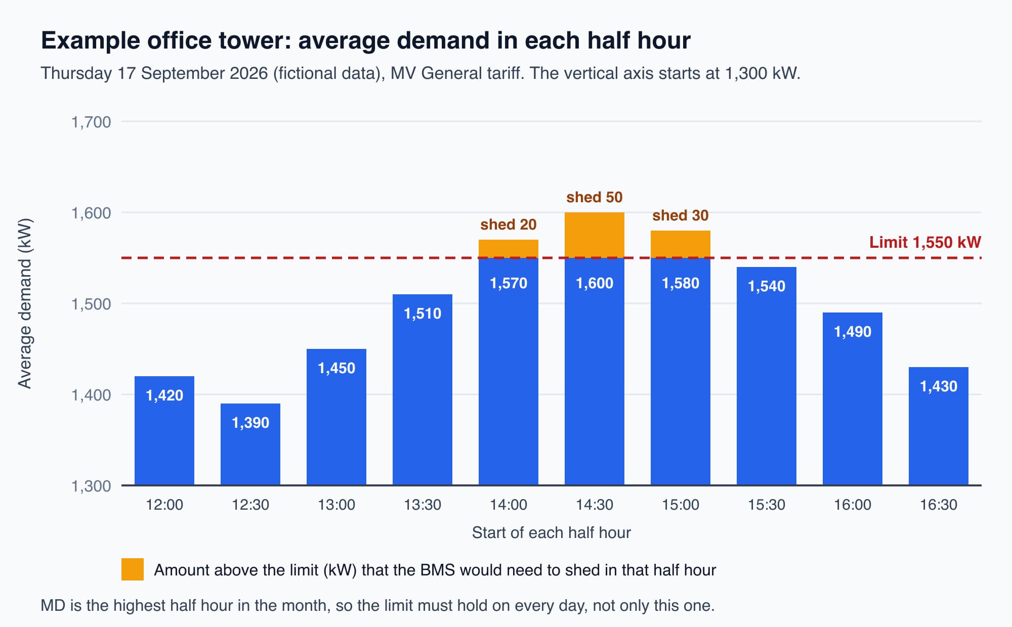
To hold 1,550 kW that day, the BMS would have needed to trim three half hours: by 20, 50 and 30 kW.

The demand charge on this bill was 1,600 kW × RM89.27 = RM142,832. If the BMS had held every half hour of the month at or below 1,550 kW, the charge would have been 1,550 × RM89.27 = RM138,368.50, a saving of RM4,463.50 for that month.

The BMS forecasts each half hour and acts before it ends

To do this, the BMS needs a power meter it can read on the building's incoming supply. It then does simple arithmetic throughout each half hour:

1. It adds up the kWh used so far in this half hour.
2. It estimates the kWh for the minutes left, assuming the present power continues.
3. It adds the two and turns the total into a half-hour average.
4. If that forecast is heading above the limit, it acts now, while there are still minutes left to pull the average down.

A worked example with the 1,550 kW limit: 1,550 kW averaged over half an hour is 775 kWh. Twenty minutes into the half hour, the meter shows 520 kWh used, and the building is drawing 1,650 kW. If that continues for the last 10 minutes, it adds 1,650 × 10 ÷ 60 = 275 kWh, for a total of 795 kWh, which is an average of 1,590 kW. That is over the limit. To stay at 775 kWh, the last 10 minutes can use only 255 kWh, which is an average of 1,530 kW. So the BMS must shed about 120 kW for the rest of the half hour.

Acting after the half hour has ended is too late. Once a half hour closes above the limit, that is the new maximum for the month.

Two practical points. The building's own meter and TNB's meter may not start their half hours at exactly the same moment, so set the BMS limit with a margin below the level you want to avoid. And check that the meter reading reaches the BMS reliably (Part 10 covered scaling, timestamps and stale data). A limit built on a frozen reading does nothing.

Demand limiting sheds loads in order from a priority list

Demand limiting is the strategy: keep each half-hour average under the limit. Load shedding is the main tool: when the forecast is too high, the BMS temporarily switches off or eases loads that can wait.

The BMS decides what to shed from a priority list, which the facility team writes and the BMS follows:

• Shed first: loads nobody will notice for a few minutes. Examples are a decorative fountain pump, a bank of water heaters, car-park ventilation fans (only while the car park's air quality allows it), and a small nudge to zone cooling setpoints.
• Shed later, if needed: larger cooling loads. In the office tower, the chiller plant uses about 35% of the building's electricity, so this is where most of the sheddable kW sits. Many chillers accept a signal that limits how much power they may draw.
• Never shed: life-safety systems, lifts, the server room and any critical process equipment.

When the forecast rises towards the limit, the BMS works down the list, starting with the least important loads and moving on only if the forecast is still too high. When the next half hour starts and there is room again, it restores the loads in reverse order, in stages. Restoring everything at once can cause a new peak, because each load comes back hungry.

A small setpoint relaxation is often the most useful shed in a tropical building. The BMS lets the zones served by AHU-12A drift up by half a degree for a few minutes. Each VAV box closes a little, the static pressure reset from Part 13 lets the fan slow down, and the chilled water load falls. A large air-conditioned floor holds its temperature for a while, so a short trim usually goes unnoticed. This is a much smaller change than the unoccupied setback in Part 7, which lets an empty building warm up overnight.

Duty cycling and staggered starts spread the load out in time

Two more tools lower the peak by changing when equipment draws power, rather than switching it off for long.

Duty cycling takes turns. If the building has several similar units, such as four cooling tower fans or a bank of small units, the BMS runs them in a rotating pattern of a few minutes on and a few minutes off, so they are not all drawing power at once. The total work stays about the same, but less of it happens at the same moment. Rotating which unit rests also spreads out wear.

Staggered start-up brings large equipment on one item at a time instead of all together. The reason is easy to get wrong. The high current a large motor draws in its first seconds lasts only seconds, so it adds very little to a 30-minute average. The larger problem is what happens next. When a building has warmed up overnight, every chiller, pump and AHU that starts together runs at full output for a long time to cool it down, and that pull-down period can last well over half an hour. Starting them in steps, with a pause between each, spreads the pull-down load and lowers the half-hour average. (Large centrifugal chillers are often started through a drive or soft starter rather than thrown straight onto the supply.)

Whether a start-up peak costs money depends on the tariff:

• MV General (the office tower): a morning start-up at 7:30am counts like any other half hour. If the pull-down is the highest half hour of the month, it sets the MD.
• MV ToU: a morning start-up before 2pm is off-peak and does not set the billed MD. The risk moves into the peak window, for example a second chiller staging on at 2pm on a hot afternoon, or the whole plant restarting after a power dip at 3pm. Those are the moments to stagger.

What demand limiting is worth, and what it is not

On the office tower's MV General tariff, each kW of maximum demand costs RM89.27 a month. Trimming the 50 kW from the earlier example is worth RM4,463.50 in a month, and RM53,562 over a year if the building holds the lower limit every month. On an MV ToU tariff, the same 50 kW would be worth 50 × RM97.06 = RM4,853 a month, but only if the trim happens inside the 2pm to 10pm weekday window.

Three limits keep these numbers honest:

• Demand and energy are separate charges. Shedding a load for a few minutes saves little energy, and some of it comes back later as the load catches up. Trimming the peak and trimming total kWh are two different savings on two different lines of the bill.
• The strategy decides the saving. A BMS has no view of your tariff. It reports demand half hour by half hour, and it carries out the strategy you set. The facility team decides which loads may be shed, where to set the limit and how far a setpoint may drift. Set the limit too low and the building runs short of cooling; set it too high and nothing is saved.
• Comfort comes first. A demand limit that leaves tenants warm every afternoon will be overridden, and an overridden limit saves nothing (Part 8 covered overrides).

None of this needs new equipment in a building that already has a BMS and a power meter it can read. It needs a known peak, a sensible limit and a clear priority list.

Worth knowing: Maximum demand is the single highest half hour of the month, so a limit that holds on 29 days and fails on one afternoon saves nothing. The BMS has to hold the limit every day, which is why a clear priority list and a margin below the limit both matter.

What comes next

Parts 12 to 14 have described what a well-set-up BMS should do: run the plant, run the air side and hold down demand. The next part, Proving the BMS Works: Commissioning and Handover, turns AHU-12A's sequence into tests you can watch and sign. It answers this question: how does anyone know the BMS actually does all this before the building's owner accepts it from the contractor?

Check your understanding

1. A building on MV ToU has its highest demand of the month at 8:00am to 8:30am on a Monday, when the plant starts. Does staggering that start-up lower its demand charge? No. On MV ToU, only half hours from 2pm to 10pm on weekdays count for the demand charge, so an 8am peak is not billed as MD. The building should look instead at its highest half hour inside the peak window. On MV General, like the office tower, the same 8am peak would count and staggering would help.
2. Twenty minutes into a half hour, the forecast says the average will be 1,590 kW against a 1,550 kW limit. Why must the BMS shed more than 40 kW? Only 10 minutes are left to pull down an average that covers the whole 30 minutes. The first 20 minutes cannot be changed, so the last 10 minutes must make up the difference. In the forecasting example, the building had to drop from 1,650 kW to about 1,530 kW, a shed of about 120 kW, to bring the half-hour average down to 1,550 kW.

Recap: A demand charge applies only on some tariffs. MV General counts any half hour at RM89.27/kW, MV ToU counts only 2pm to 10pm on weekdays at RM97.06/kW, and LV has no per-kW charge. Maximum demand is the highest metered 30-minute average in the month, so a BMS forecasts each half hour and sheds loads from a priority list before the half hour ends. Setpoint relaxation, duty cycling and staggered starts lower the average without much loss of comfort. The limit has to hold every day of the month, and the BMS only carries out the strategy the facility team sets.

Go deeper on video (optional)

This video explains demand charges and ways to shave a peak. It comes from outside Malaysia, so its interval length and the hours when demand counts may differ from TNB's; for Malaysian bills, use the tariff and maximum demand rules above. It is optional; you do not need it for the next part.

This is Part 14 of 16 in Cobler's Building Automation and BMS Fundamentals course. Previous: How a BMS Runs the Air Side: VAV, Static Pressure Reset and Fresh Air. Next: Proving the BMS Works: Commissioning and Handover.

Cobler builds CobiNeural, a platform that shows a facility team its building's energy, water and indoor air data as live numbers across the whole site. To see how your building performs, talk to us.