Why Chiller Efficiency Is Measured at Part Load: Understanding IPLV

Part 15 of 20 in Cobler's Cooling Fundamentals course. New here? See the course page.

Part 14 ended on a gap. Every chiller comes with a headline efficiency figure on its nameplate, something like 0.60 kW/RT, but that figure is measured at full load, with the chiller delivering 100% of its rated cooling on a design day. Most of the time a chiller runs well below that. So if full load is rare, what is a chiller's efficiency the rest of the time?

This part answers that question. We look at how much of its life a chiller spends at part load, how its efficiency changes there, and how a figure called IPLV combines those part-load results into one number. It builds on Part 13, which explained kW/RT (lower is better) and COP (higher is better).

(If your building has only split units and cassettes, like the shoplot, you can skim this part. The idea that efficiency changes with load applies to your units too, but IPLV and chiller staging apply to chilled-water plants.)

What part load means

Full load means the chiller is producing all the cooling it was designed for. Part load means it is producing less, for example 60% of its capacity on a mild, cloudy morning instead of 100% on a very hot afternoon.

A chiller is sized for the worst case: the hottest, fullest hour of the year, so that the building still stays cool on that afternoon. Every other hour, the building needs less cooling than the chiller can give, so the chiller turns itself down. Oversizing, which is common, pushes it even further down.

The office tower shows this. It has three 500 RT chillers, two on duty and one on standby, so 1,000 RT of duty capacity. Its peak cooling load is about 900 RT. Even at that peak, the two duty chillers are at 90% load. On most hours they run lower.

How a chiller's hours are usually weighted

How much time does a chiller spend at each load? The AHRI 550/590 standard, the North American rating standard most of the industry uses for chillers, weights a chiller's operation like this:

• 100% load: about 1% of the time
• 75% load: about 42% of the time
• 50% load: about 45% of the time
• 25% load: about 12% of the time

In this weighting, the full-load condition on the nameplate counts for about one hour in a hundred.

These percentages are the standard's weighting assumptions, not a measured duty cycle for your building. AHRI chose them so that every manufacturer calculates the same blended figure in the same way, and the results can be compared fairly. Your building's real profile might lean heavier or lighter, depending on its occupancy, its use and the local climate. In Malaysia, where the cooling load never switches off, the profile looks different again from a temperate office block. But the main point holds everywhere: part-load hours dominate, and full load is rare.

So part-load efficiency decides most of your real energy use, and a single full-load figure leaves most of it out.

IPLV, one figure that weights the part-load results

IPLV (integrated part load value), defined in AHRI 550/590, takes the chiller's efficiency measured at four load points (100%, 75%, 50% and 25%) and combines them into one figure, using the weights from the previous section. A useful comparison is a student's grade-point average: instead of judging the student on one exam, each subject counts according to its weight. IPLV judges the chiller on all four load points, not only on full load.

How you combine the four results depends on which efficiency unit you use.

If the four results are in kW/RT, the standard uses this form:

$$\text{IPLV} = \frac{1}{\dfrac{0.01}{A} + \dfrac{0.42}{B} + \dfrac{0.45}{C} + \dfrac{0.12}{D}}$$

where A, B, C and D are the chiller's kW/RT at 100%, 75%, 50% and 25% load, and 0.01, 0.42, 0.45 and 0.12 are the weights shown earlier.

If the four results are COP (or EER, where higher is better), the standard uses a plain weighted sum:

$$\text{IPLV} = 0.01A + 0.42B + 0.45C + 0.12D$$

where A, B, C and D are now the COP values at 100%, 75%, 50% and 25% load.

Both forms give the same answer once you convert between kW/RT and COP (the box at the end explains why there are two). Two rules follow:

1. Use one unit throughout. A, B, C and D must all be kW/RT, or all COP. Mixing units gives a meaningless number.
2. Use the matching formula. The reciprocal form is for kW/RT only. Putting COP values into it, or adding kW/RT values with the plain weighted sum, gives the wrong result.

A worked example

Suppose a water-cooled chiller measures:

• A = 0.60 kW/RT at 100% load
• B = 0.55 kW/RT at 75% load
• C = 0.52 kW/RT at 50% load
• D = 0.58 kW/RT at 25% load

This machine is more efficient in the middle of its range than at full load. The next section explains why. Using the kW/RT form:

$$\text{IPLV} = \frac{1}{\dfrac{0.01}{0.60} + \dfrac{0.42}{0.55} + \dfrac{0.45}{0.52} + \dfrac{0.12}{0.58}} \approx 0.54 \ \text{kW/ton}$$

Working it through: 0.01 ÷ 0.60 = 0.017, 0.42 ÷ 0.55 = 0.764, 0.45 ÷ 0.52 = 0.865 and 0.12 ÷ 0.58 = 0.207. These add up to about 1.853, and 1 ÷ 1.853 is about 0.54 kW/RT.

You can check this with the COP form. Converting each point with COP = 3.517 ÷ kW/RT gives COPs of about 5.86, 6.39, 6.76 and 6.06. The weighted sum is 0.01 × 5.86 + 0.42 × 6.39 + 0.45 × 6.76 + 0.12 × 6.06, about 6.5, and 3.517 ÷ 6.5 is about 0.54 kW/RT, the same answer.

So the full-load nameplate says 0.60 kW/RT (a COP of about 5.9), but the IPLV of about 0.54 kW/RT (a COP of roughly 6.5) better reflects a typical year under the standard's assumptions.

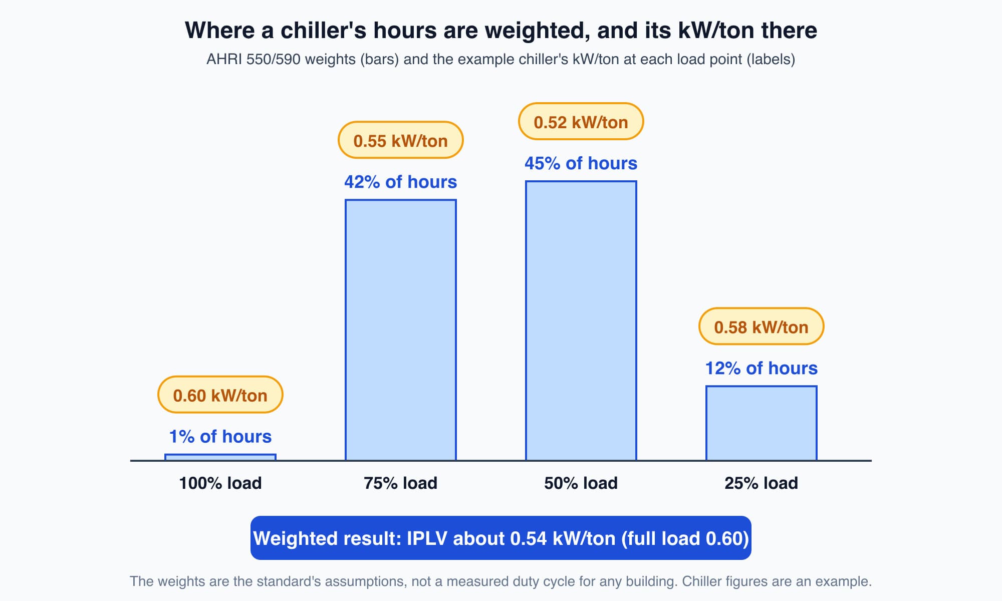
The example chiller's kW/RT at each load point, with the AHRI weight for each point; the 75% and 50% points carry most of the weight.

You will also meet NPLV (non-standard part load value). It uses the same method, but at your site's own conditions (your actual condenser-water temperatures, for example) instead of AHRI's standard conditions. IPLV is the catalogue figure for comparing machines. NPLV is the figure for your plant.

Why part load can be more efficient: condenser relief

You might expect a chiller at part load to waste energy, like an idling car engine. Often the opposite is true: many chillers have a lower (better) kW/RT at 50 to 75% load than at 100%. The reason is the temperature of the condenser water.

As Part 2 explained, the compressor's job is to take heat from the cold side (the chilled water) and lift it to the warm side (the condenser), where the cooling tower carries it away. The bigger the temperature gap between the two sides, the higher the pressure the compressor must lift the refrigerant to, and the more electricity it uses for each ton of cooling.

A chiller is usually at part load because the day is milder. On a milder day, the cooling tower can often send back cooler condenser water. Cooler condenser water means a smaller lift, so the compressor does the same cooling with less electricity. This effect is called condenser relief. The AHRI part-load test points also assume cooler condenser water as the load falls, so condenser relief is built into a chiller's published IPLV.

There is a limit, and it matters in Malaysia. As Part 12 explained, a tower cannot cool water below the outdoor wet-bulb temperature, and here the wet-bulb temperature stays fairly high all year. So on your site, the condenser water may not get much cooler at part load, and the part-load gain can be smaller than the IPLV suggests. That is exactly what NPLV, or a measured figure, captures.

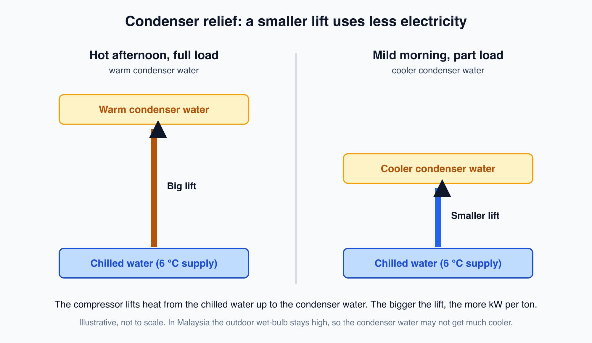
The compressor lifts heat from the chilled water up to the condenser water; cooler condenser water means a smaller lift and less electricity per ton.

The efficiency usually falls again at very low load. In our example, the kW/RT rose to 0.58 at 25% load, because the chiller's fixed losses are spread over much less cooling. So the best region is usually the middle to upper part of the range, with cool condenser water, not the very bottom.

How a chiller turns itself down

To run efficiently at part load, a chiller must modulate, meaning adjust its capacity smoothly, rather than switch on and off. There are two main ways:

• Inlet guide vanes on centrifugal chillers: adjustable blades that control how much refrigerant vapour enters the compressor.
• Variable compressor speed: the compressor slows down when less cooling is needed.

Variable speed uses a variable-speed drive (VSD, also called a VFD or inverter), which changes the frequency of the supply to the motor so the motor can run at any speed. Rectifiers and inverters explains how the drive builds that variable-frequency supply, and how electric motors work explains why motor speed follows frequency.

How much power does slowing down save? It depends on the machine:

• For a fan, or a pump in a closed loop with no fixed pressure to hold, power falls roughly with the cube of speed, as Part 9 showed: at 80% speed it needs roughly half the power.
• A compressor is different. It must always lift the refrigerant from low pressure to high pressure, and the size of that lift is set mainly by the chilled-water and condenser-water temperatures, not by the compressor's speed. So a compressor's power does not follow the cube law. A variable-speed compressor saves most when the lift is also smaller, for example when the condenser water is cooler (see the section on condenser relief).

That is why variable-speed chillers often post strong IPLV figures: the standard's part-load points come with cooler condenser water, where variable speed pays off best. At your site, the gain depends on how cool your condenser water really gets.

Staging: how many chillers to run

A single efficient chiller is only part of the plant. Most large buildings have several chillers, and the controls decide how many to run and how heavily to load each one. This decision is called staging.

Take the office tower on a mild morning, with a cooling load of about 600 RT:

• Run three chillers at 40% each. Each is lighter loaded and closer to the 25% region where efficiency falls again. In plants where each chiller has its own condenser-water pump and tower cell, the third chiller also brings its pump and tower fan into service.
• Run two chillers at 60% each. Both sit in the efficient middle of their range, and the third chiller and its auxiliaries stay off.

The second option delivers the same cooling with less electricity. A plant of efficient chillers can still be an inefficient plant if it stages them badly. Part 18 looks at oversizing, short-cycling and staging problems, and Part 19 shows how the building management system (BMS) makes staging decisions.

Worth knowing: Two chillers with identical full-load nameplates can have very different IPLVs. Judged on its nameplate alone, the chiller in the worked example would look worse than it is, so compare chillers on IPLV, or on NPLV at your own site's conditions.

Optional detail: Why are there two forms of the IPLV formula? The standard averages the cooling delivered per unit of electricity at each load point, which is what COP measures. With COP values you can weight and add them directly. A kW/RT value is the upside-down version of that ratio, so the kW/RT form first turns each value upside down (0.01 ÷ A and so on), adds them with their weights, and then turns the total back into kW/RT with the "1 ÷" at the front.

What comes next

A chiller's real kW/RT changes with load, condenser-water temperature and the slow fouling of its heat exchangers. A nameplate or an IPLV cannot tell you what your plant is doing today. Part 16 explains what to measure (flow, temperature and power) and how to prove that a change has saved energy. It answers the question: how do you find out how well your cooling is really performing?

Check your understanding

1. A chiller's kW/RT values at 100%, 75%, 50% and 25% load are all 0.60. What is its IPLV? 0.60 kW/RT. With the kW/RT form, 0.01 ÷ 0.60 + 0.42 ÷ 0.60 + 0.45 ÷ 0.60 + 0.12 ÷ 0.60 = 1.00 ÷ 0.60, and 1 divided by that gives 0.60. The weights add up to 1, so equal values give the same value back.
2. Why might a chiller in Malaysia gain less at part load than its IPLV suggests? Much of the part-load gain comes from cooler condenser water (condenser relief), and the AHRI test points assume it. Here the outdoor wet-bulb temperature stays high all year, so the tower may not deliver much cooler water at part load, and the gain is smaller.

Recap: A chiller's full-load nameplate describes a condition that, in AHRI's weighting, it sees about one hour in a hundred. IPLV combines its efficiency at 100%, 75%, 50% and 25% load with weights of 1%, 42%, 45% and 12%. With kW/RT values, use the reciprocal form; with COP values, use the plain weighted sum. NPLV does the same at your site's conditions. Part load is often more efficient because of condenser relief, but the gain depends on cool condenser water and fades at very low load. The cube law applies to fans and pumps without static head, not to compressors. Staging decides whether a plant keeps its chillers in their efficient range.

Go deeper on video (optional)

This video explains why a chiller's full-load figure does not reflect real operation, and how IPLV and NPLV weight part-load performance. It covers the same ideas as the sections on weighting, IPLV and the worked example. You do not need it for the next part.

This is Part 15 of 20 in Cobler's Cooling Fundamentals course. Previous: Why Air Conditioning Is the Biggest Line on a Malaysian Building's Electricity Bill. Next: BEI Malaysia: Scoring Your Building's Cooling by Measuring It.

Cobler builds CobiNeural, a platform that shows a facility team its building's energy, water and indoor air data as live numbers across the whole site. To see how your building performs, talk to us.