Current Transformers and Power Meters

Part 19 of 23 in Cobler's Electricity Fundamentals course. New here? Start with the course map.

Let's go back to the busbar leaving one of the office tower's transformers. At full load it carries 2,165 A. Now the meter that reports that current takes in at most 5 A, over the same size of wire as a socket circuit, and the two are never electrically connected. Between them sits a ring of iron wound with thin wire. So how does a current transformer work? Well, it's basically the transformer of Part 9, wound inside out, and once we see that, every sub-meter in a building starts to make sense.

In Part 18 we mapped the tree from the 11 kV intake to every load, and we ended at its blind spot. The TNB (Tenaga Nasional Berhad) meter sees the whole tree as one number. So to manage the building, we need a number for every branch, measured on live copper without cutting into it.

How does a current transformer work?

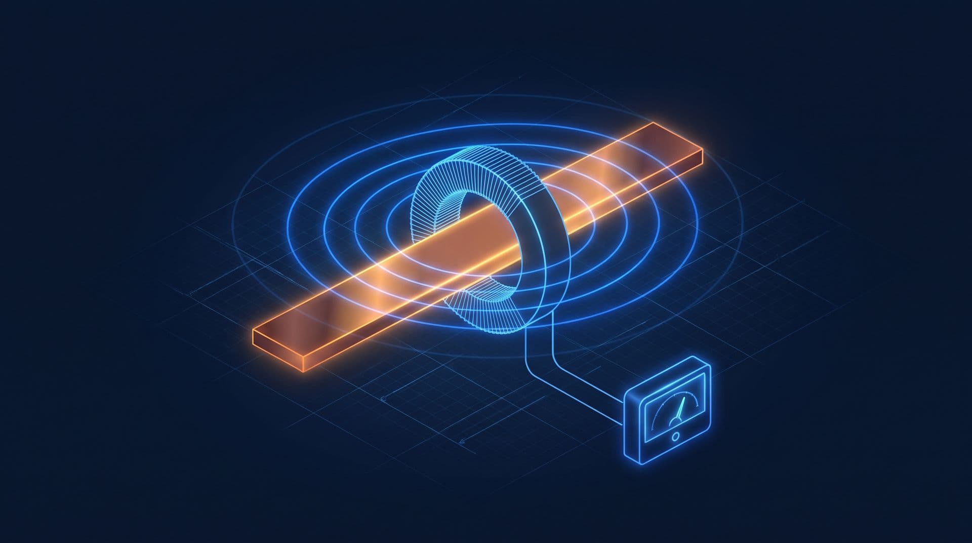
Imagine an iron ring with the busbar passing once through the middle, and hundreds of turns of thin wire wound around the ring itself. Let's follow what happens. The alternating current in the busbar makes a magnetic field that circles it, as Oersted found in Part 6. The iron ring gathers that field into a loop of flux. Because the current alternates, the flux keeps changing, and by Faraday's law from Part 7 it induces a current in the secondary turns.

So what we've built is a transformer whose primary winding is the cable or busbar itself, passing once through an iron ring, and whose secondary is hundreds of turns of thin wire wound on that ring. That's what we call a current transformer (CT).

Now Part 9 gave us the rule for transformers. Voltage goes with the turns, and current goes the other way. For a CT we write it as a balance of ampere-turns:

$$N_p I_p = N_s I_s$$

Let's take a 2000/5 CT. It has one primary turn carrying 2,000 A, so 1 × 2,000 = 400 × 5, which means the ring carries 400 secondary turns. It's kind of like a see-saw, with a heavy adult near the pivot (2,000 A on one turn) balanced against a small child far out (5 A on 400 turns). At 1,000 A in the busbar the secondary carries 2.5 A, and at 100 A it carries 0.25 A. The meter just multiplies back by the ratio, 400, and shows the busbar current.

But why does the small current copy the big one so faithfully? Well, the secondary current makes its own field, and that field pushes against the primary's (Lenz's law, Part 7). The two almost cancel. The core keeps only a small leftover flux, just enough to induce the voltage that drives the secondary current around the meter circuit. If the busbar current rises, the leftover grows and induces a little more, and the secondary current rises to match.

Two things follow from this. The meter wiring never touches the 400 V copper, because only the magnetic field links them. And a CT works only on AC (alternating current). A steady DC (direct current) makes a steady field, which induces nothing, exactly as Part 9 found for transformers.

Open and shorted secondaries

Now this next bit felt kind of backwards to me at first. Everywhere else in this course, an open circuit is the safe state, like Part 4's open switch that stops the current. With a CT it's the other way round, because the secondary current is what keeps the core calm. Take it away and the CT becomes a high-voltage generator. To see why, let's look at the voltage on the secondary.

In normal running that voltage is tiny. The CT only has to push 5 A through the meter input plus the wires, and we call that load its burden. Say we have 10 m of 2.5 mm² copper wire in all (5 m out, 5 m back). Using \(R = \rho L / A\) from Part 3:

$$R = \frac{(1.68 \times 10^{-8}) \times 10}{2.5 \times 10^{-6}} \approx 0.067\ \Omega$$

At 5 A that's 5 × 0.067 ≈ 0.34 V, and 5² × 0.067 ≈ 1.7 VA of burden, so the whole reading for 2,000 A travels on less than half a volt.

Now imagine we unplug the meter while the busbar is live. The secondary current stops, so nothing cancels the primary's 2,000 ampere-turns, and all of it magnetises the core until the core saturates. Then twice every cycle, as the busbar current swings through zero, the flux flips from fully saturated one way to fully saturated the other in a very short time. We know from Faraday's law that the induced voltage is the number of turns times how fast the flux changes. So 400 turns times a sudden flip gives spikes that can reach several kilovolts on a large CT (Schneider Electric). That's enough to arc across the terminals, break down insulation, start a fire or kill someone.

So for a CT, the safe idle state is actually shorted. Current keeps circulating and the voltage stays near zero. That's why metering panels have shorting test blocks, and the rule is to short the CT before disconnecting anything. And it's the exact opposite of a voltage transformer, which must never be shorted. We can lay out all the cases side by side:

Solid-core, split-core and Rogowski coils

Now a closed ring means unbolting the busbar to thread it through. So how do we meter a board that's already built and live? Well, what if the ring opens on a hinge? Or what if we drop the iron altogether, and the saturation with it? That gives us three forms, each with its own trade-offs:

• Solid-core CTs are closed rings. They're the most accurate, but the busbar must be disconnected to thread through, so they suit new switchboards.
• Split-core CTs open on a hinge and close around a cable, so a board can be metered without being rebuilt. The joint leaves a tiny air gap that slightly weakens the coupling, though revenue-grade split-cores exist (CT ratios and specs). Fitting one still means working near live parts, which is a job for a competent person.
• Rogowski coils are flexible loops with no iron at all. Their output voltage follows the rate of change of the current (Faraday again), so an electronic integrator turns it back into a current reading (PEM). With no iron there's nothing to saturate, the loop wraps around big or awkward busbars, and its small output voltage isn't dangerous if left open. The price is the powered electronics.

And we've actually met CTs already. The AC clamp meter from Part 2 is a split-core CT in a handle. The residual current device of Part 14 is one too, with live and neutral passing through the same ring, so it only sees their difference.

Every CT also has an accuracy class. A class 0.5 CT keeps its ratio error within 0.5 percent at 100 to 120 percent of its rated current, 0.75 percent at 20 percent and 1.5 percent at 5 percent. Below 5 percent the class doesn't specify it at all (Beckhoff). Class 0.5S extends the specified range down to 1 percent of rated current (Schneider Electric). That's why a CT should be sized so its normal load sits well inside its range.

The power meter

So now the meter has a small copy of the current. How does it get from that to kW and kWh? Well, a multifunction meter, also called a digital power meter (DPM), takes two inputs per phase. One is the voltage, through small fused leads (or a voltage transformer at 11 kV), and the other is the current from the CT. It samples both thousands of times a second and multiplies each pair to get the power at that instant. That's \(P = VI\) from Part 5, now at every instant. Then it averages over each cycle:

$$P = \frac{1}{N} \sum_{k=1}^{N} v_k \, i_k$$

But why average the products, instead of just multiplying the two readings? Well, when the current lags the voltage, as in Part 12, part of each cycle has the voltage and current pointing opposite ways. Those products come out negative, which is energy flowing back to the supply. That means the average of the products counts only the real power, in kW. The RMS (root mean square, the heating-equivalent value) voltage times the RMS current gives the apparent power in kVA, and kW ÷ kVA is the power factor.

From there the meter keeps running totals. Adding up kW over time gives kWh, and the highest 30-minute average gives maximum demand (both Part 5). If we run the same samples through a Fourier calculation, the meter also reports total harmonic distortion (THD), the distortion measure of Part 16. A modern revenue meter at the intake does the same arithmetic under a utility seal, and How Electricity Meters Work tells its story from spinning disc to smart meter.

Sub-metering

Now if we fit a CT set and a meter to each feeder, the tree from Part 18 gets its numbers, and that's what we call sub-metering (what it finds). It does three jobs:

• Attribution: which feeder made the 3 pm peak, which one runs all night.
• A sum check: the feeders should add up to the incomer, less small losses. A gap points to a CT on the wrong cable, a reversed CT or a wrongly programmed ratio (the checklist).
• Honest error bars: the CT's error and the meter's error stack up. That, plus different measurement points and demand windows, is why a sub-meter never matches TNB's meter exactly.

The chiller plant feeder

So let's go back to the office tower. The main switchboard (MSB) feeder to the chiller plant peaks at about 720 kW (Part 18's table). At 400 V and a power factor of 0.9, the current is:

$$I = \frac{P}{\sqrt{3} \times V \times \text{PF}} = \frac{720{,}000}{1.732 \times 400 \times 0.9} \approx 1{,}155 \text{ A}$$

A common rule is to add 25 percent and round up to a standard ratio, which gives us 1500/5. The tower's already built, so the contractor fits three split-core class 0.5S CTs, one per phase (an illustrative spec). Their thin secondary wires run to a shorting test block, and then to a multifunction meter on the panel door.

Now at the 3 pm building peak, the feeder carries about 1,123 A per phase. Each CT sends 1,123 × 5 ÷ 1,500 ≈ 3.74 A to the meter, which multiplies by 300 and reads 1,123 A. Per phase, real power is 230 V × 1,123 A × 0.90 ≈ 232 kW, so the three phases total about 697 kW, which is the 700 kW in Part 18's table. Apparent power is 3 × 230 × 1,123 ≈ 775 kVA, and 697 ÷ 775 gives a power factor of 0.90.

That puts the CT at 75 percent of its rating, comfortably inside its accurate band. But at 2 a.m., with one pump on, the feeder may carry 30 A (illustrative), which is just 2 percent of the CT's rating. A plain class 0.5 CT is unspecified there. The 0.5S CT is still specified, to within 1.5 percent at worst, so the night-time waste shows up honestly. And that's the trade-off behind the spec. A CT small enough for the 2 a.m. load would be overloaded at the afternoon peak, so we size the CT for the peak and let the S class keep it accurate at night.

The same is done for every chiller, pump and cooling tower fan. The plant room ends up with about thirty meters (illustrative), each one holding its own numbers in its own box. CobiNeural reads digital power meters like these and shows each branch's kW, kWh and power factor side by side.

What the meter can't see

So the chiller feeder's meter says 697 kW. But is that good? Well, electricity alone can't tell us. A chiller plant's efficiency is measured in kW per refrigeration ton (kW/RT), which is electricity in against cooling out (chiller plant efficiency). To know the cooling out, we need the chilled-water supply and return temperatures and the flow rate, and none of those is electrical. Neither is the carbon dioxide (CO2) in a meeting room.

The meter now knows the electricity. But half of what matters in a building isn't electrical, things like temperature, CO2 and flow. So how do we measure those? Part 20 shows how sensors turn them into electrical signals, and those signals into numbers.

This is Part 19 of 23 in Cobler's Electricity Fundamentals course. Previous: Building Electrical Distribution. Next: Sensors and 4-20 mA Signals.

Cobler builds CobiNeural, which reads the power meters on a building's feeders and shows every branch's kW, kWh and power factor live, with alerts before a peak sets the bill. To see it on your own switchboards, talk to us.